A time series is a sequence of numerical data points which are represented in successive order.
In Investment and Capital, a time series tracks the movement of the chosen data points, such as a security’s price, over a specified period of time with data points recorded over a regular intervals.
In Time Series there is no minimum or maximum amount of time that must be included thus allowing the data to be gathered in a way that provides the information being sought by the investor or analyst examining the activity.
Initial Environment Setup
But before we get into creating a program let’s just first set up a proper environment for R programming.
To install R programming tool go to the following link and download the software and install it.
For Windows Users:
And Type and Run the following code RGui
install.packages(“ggplot2”)
For Linux Users:
If you are on Linux platform then you can use this fast and easy command used in Linux which can be used to install R. The yum command is used for installing like this:
$ yum install R
For Ubuntu Linux or other Debian-related OSs, a more direct method is:
$ apt-get install r-base
Now Let’s Start using the RGui (64 -bit) which will be installed in the Installation folder which we had selected while installing the software.
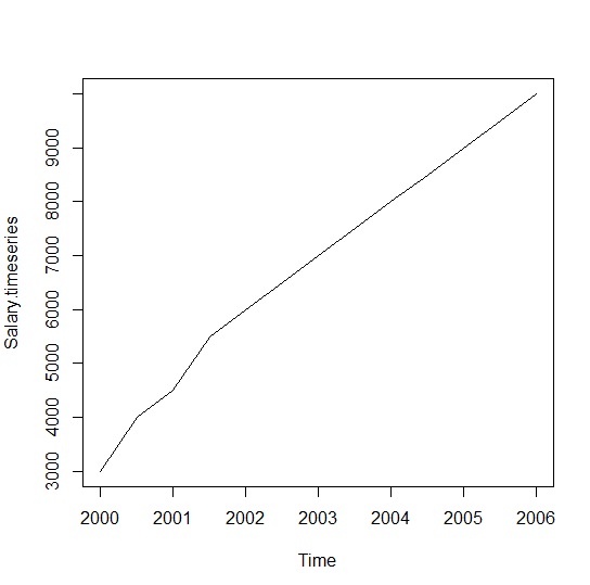
Code for Plotting a Time Series for a Salary Growth is as Follows:
Comments are presented with a # at the start
# timeseries.object.name <- ts(data, start, end, frequency)
# data is a vector or matrix containing the values used in the time series.
# start specifies the start time for the first observation in time series.
# end specifies the end time for the last observation in time series.
# frequency specifies the number of observations per unit time.
# Get the data points in form of a R vector.
Salary <-
c(3000,4000,4500,5500,6000,6500,7000,7500,8000,8500,9000,9500,10000)
# Convert it to a time series object.
Salary.timeseries <- ts(Salary,start = c(2000),frequency = 2)
# Print the timeseries data.
print(Salary.timeseries)
# Plot a graph of the time series.
plot(Salary.timeseries)
# Give the chart file a name.
png(file = “Salary.png”)
# Save the file.
dev.off()
Output for the above Code:
Syllabus of Data Science training in Mumbai


